I was continuing from the last post. I will explain why I picked the paper I did, answer the questions from the previous post, and show my note-taking and thought process. After reading hundreds if not thousands of whitepapers, blogs, or articles, this is my distilled version of how I approach it. I will document this for the first time. It may be different from how others approach it. Over time you will get your own approach. So let’s hit the stacks.

Disclaimer: Not financial advice, only my own opinions. This is not to encourage nor promote taking any trades, positions, or investments of any kind. Any information contained in this website is for informational purposes only and to be taken as is. DWongResearch and the Author (Derek Wong) has done their best to ensure accurate information. Regardless of anything contrary, nothing available on this website should be understood as a recommendation, consult a licensed financial professional in your jurisdiction.

Selection

After reading both articles, Using an unsupervised machine learning algorithm to detect different stock market regimes by Ethan Johnson-Skinner, over The Search for Crisis Alpha: Weathering the Storm Using Relative Momentum By Nathan Faber of Newfound Research, I found them equally intriguing. Again we come back to the dichotomy of something I think will be helpful (Crisis Alpha) or something that will push the limits of my knowledge (Machine learning and Gaussian mixture models). While reading them both, I was indifferent. One thing that was abundantly clear on replication was the data complexity of the Faber paper.

The data required for replication is complex in the Newfound paper because a few steps are laid out in a footnote on page 6 (Yes, you have to read the footnotes). Specifically, you need to create constant maturity indices Damadaraon style except for the 7 year, which starts only in 1969 when the rest start in 1962. Then from 1987 January to 1993 September, the 20 year bond did not trade. So at the get-go, you are already making a lot of data assumptions and proxies when in the end, you would like to use a table of fixed income ETFs (SHY, IEI, IEF, TLH, and TLT), which are relatively young compared to the constant maturity indexes we measure against.

I think that this paper deserves more attention and may come back to it in the future. For this series of articles, the complexity of the idea is not as important as the ability for a reader to follow along. The other paper by Johnson-Skinner comes with python code (I have not tested it yet) and uses simply accessible data sources as far as I could tell when looking at the data requirements.

So diving into Using an unsupervised machine learning algorithm to detect different stock market regimes, we go.

Notes and Highlights

So the first thing I do is highlight liberally. It seems almost like I copied the entire article, which is not long. But each of these pieces will give me a point of information to interact with. I even highlight things that seem repetitive to I already know. The reason is it will keep context if I ever need to go back. I store all of these highlights and notes in a digital platform that is searchable to if I ever come back later, it is easy.

You can skip this part and go to the [next section](## Gathering Resources) if you wish. It is maybe a bit bland.

The top bullet point is the direct quote followed by my thoughts while reading it.

• The Gaussian Mixture model (GMM) will be used to detect different moods in the stock market. The GMM model will be applied twice: first using price data, and subsequently with macro-economical data.

• • For the setup, we have 2 experiments. One with price data only (single feature) and another with additional macro-economical data (2 features)

• The difference between the two approaches is the use of labeled datasets: supervised learning uses labeled input and output data, whereas an unsupervised learning algorithm does not.

• • Definition of supervised vs. unsupervised learning. We will not need any labeling because this method is unsupervised.

• The gaussian mixture model is the overlapping of multi-normal distributions in p-dimensional space. The dimension of the space is generated by the number of variables.

• • Definition of what a GMM is, simply a collection of multiple Gaussian distributions that overlap in p-dimensional space.

• For example, if we had one variable (S&P 500 returns), the GMM would be fit based one dimensional data. The GMM can be used to model the state of the stock market along with other financial applications. One characteristic from the stock market returns, is heavy tails, which are generated from days of high volatility. The ability to capture highly volatile days in the tails of the distribution is important for capturing information in the modelling process.

• • GMM allows for the capture of heavy tails generated by dates of high volatility. This is an advantage over a standard gaussian.

• One main benefit of using the GMM for unsupervised clustering is the space encompassing each cluster can take on a ellipse shape. Gaussian mixture models take not only means into account but also covariance to form a cluster.

• • Each cluster takes on an ellipse shape, and the mixture model will also take into account covariance.

• it can be hard to put intuition behind the resulting market conditions.

• • The classic machine learning excuse is that we cannot intuit the reasoning behind a black box.

• The goal of the Gaussian Mixture Model is to assign data points to one of n multi-normal distributions. To do this, an Expectation Maximization (EM) algorithm is used to solve the parameters of each multi-normal distribution.

• • We are going to solve using Expectation Maximization. So whats that? Quick google search and A Gentle Introduction to Expectation-Maximization (EM Algorithm)
  • After reading some background information, I can now see that it is a Maximum Likelihood Estimation.

• Step 1: Randomly initialize the starting normal distribution parameters

• Step 2: Preform the E-step or the expectation step

• Step 3: Preform the M-step of the maximization step

• Step 4: Calculate the log likelihood of the joint probability of (Data given fraction of each state , mean , covariance)

• Step 5: Repeat steps 2–4 until the log-likelihood converges

• • This part is critical, it is the algorithm used to solve the parameters. We will need this later, but it also builds on the link I referenced, which describes the E-step and M-Step in more detail.

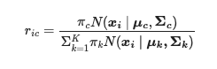
• The probability that each data point belongs to a certain cluster is given below. Based on the indexing, we are given a probability of each data point belonging to each induvial cluster.

• Since it is a probability matrix, the values will sum to 1 under index ‘i.’

• 

• The interpretation is as follows: the index i represents each data point or vector. The index c represents that given cluster; if we were to have three clusters (c) would be 1 or 2 or 3.

  • This is where knowing mathematical notation and coding comes in handy. We are going to need to break up the formula into parts that we can understand.

  • First what is N?

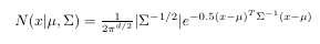
    • The multivariable Gaussian formula is given where mu and sigma are parameters that require estimating using the EM algorithm.

  • So the numerator is $\pi_c$, what the heck is this? So I am inferring here using my prior knowledge but I could be wrong. It was giving that this is an element of a probability matrix. So this value is a probability so $r_{ic}$ must be the probability that $x_i$ is generated by cluster $c$. Hence in a Bayesian framework $\pi_c$ must be a prior estimate of component $c$.

  • the $\Sigma$ means we are going to have to iterate from $k=1$ to $K$ for all estimates of $\pi_k$ which should sum to 1 assuming a uniform distribution prior.

  • Honestly its a boatload of inference here, but this is my first time with GMMs so please bare with me. I could also be wrong as using this paper along does not give a formal definition.

  • So basically in mathematical terms we will calculate $$ \forall i,c\
    r_{i,c}=\frac{\pi_c \mathcal{N}(x_i | \mu, \Sigma_c)}{\Sigma^{K}_{k=1}\pi_k\mathcal{N}(x_i |\mu_k, \Sigma_k)} $$

  • In programming terms we are going to have 3 loops as far as I can see now. One each for $i$, $c$, and $k$. stored in a matrix of size ($i$, $c$)

• An additional key concept is that each Gaussian distribution in our space is unbounded and overlapping with one another. Based on the location of the data point, a probability is assigned to it from each distribution. The probabilities for each data point belonging to any of the clusters will sum to 1.

• • This confirms my hypothesis above, I think.

• Lastly, since the EM algorithm is an iterative process, we need to gauge the progress at each step to know when to stop. To do this, we use the log-likelihood function for the model to measure when our parameters are converging.

• • This implies that the step we did above was actually the E step and now we are in the M step. The convergence of log-likelihood is well documented.

• Here I will assume three states — BEARISH , NEURAL, BULLISH.

• • This is reasonable

• I will be using the log returns of the S&P500 to fit the GMM.

• • Log returns are always better than percent returns.

• The States for the Gaussian mixture model are found using the Gaussian Mixture model from sklearn and the input data is the daily return for the S&P500.

• • Sure let us use a sklearn, but I will check the documentation and see if the implementation is as I think the algorithm works.

• One issue that may arise is convergence. Not in the sense of meeting the criteria of a certain threshold in the EM algorithm, but rather based on the initial conditions, different distributions may take shape depending on the run. Further investigation will be required here.

• • It is always an issue with estimation

• To begin and demonstrate the GMM visually, I will use two-dimensional data or two variables for simplicity. Each corresponding cluster is a multi-normal distribution in three dimensions. In this example, the first dimension is the inflation value (let’s call this X), the second dimension is the S&P500 monthly % return (let’s call this Y) and the third dimension is the joint probability of X&Y. In other words given a certain combination of X and Y what is the probability.

• • How do you create this 3rd feature that was not explained above, unless this comes from step 4. I am not clear at this point because no formula was given.

Notes summary

My key takeaways:

• GMMs can model fat tails using purely a mix of normal distributions
• We need 2 steps to make this function the expectation and maximization steps.
• In the end, we will have 3 dimensions, was this generated by step 4? If so, how do we complete that?

Gathering Resources

• Data

• • We need SPY close data for experiment one
  • we need SPY close data and inflation data for experiment 2

We can get SPY data from yahoo finance or another free website. From the comments of the code snippets

from scipy.stats import multivariate_normal
from sklearn.mixture import GaussianMixture
#'10YrYeild':treasury_yeild.Close.values
# 0. Create dataset
sp_list = ['SPY']
symbols_list = sp_list
start = '2008-01-01'
print('S&P500 Stock download')
r = yf.download(symbols_list, start,end)
daily_returns = (r.Close.pct_change()) #Daily log returns Close price for each day -  Y observations 
daily_returns = daily_returns.iloc[1:]
X = daily_returns.values
GMM = GaussianMixture(n_components=3).fit(X.reshape(-1,1)) # Instantiate and fit the model

The code and the comments/article have an issue here. Although the report says we use inflation data and comments, it seems that the 10-year yield is the proxy. This code snippet doesn’t download that data. We are going to have to deal with that ambiguity. Often, we will see that there is critical information missing and take the bits of clues we have to piece something together.

• Code

• Python packages required:

• • pandas, NumPy, DateTime, scipy, sklearn

Mise en place

Now it is time to get everything ready. We have read the article and understand the current requirements. We have a potential place to download free data from (yahoo finance). However, we are also left with an ambiguity, where is this 10-year yield coming from and how are we supposed to use it?

Conclusion

Let’s revisit our questions from the previous article.

1. Can I understand the basic principles of why this should work?

2. 1. Yes, we use multiple Gaussians and 2 steps of expectation estimation and log-likelihood maximization.

3. What resources do I need to put together to replicate this (data, code, packages, study some background information)?

4. 1. We found a data source, and what data is required SPY and 10-year yields
   2. Code-wise, we have an ambiguity. We cannot see where there was a usage of the 10 year yield
   3. We have a package list for python code that we will need to install if we don’t have it.
   4. Yes, we needed some background information to understand this article, which was linked in the highlights section.

5. How do I replicate this as close to the paper as possible? If there are some gaps in the logic, or things are vague, what assumptions do I need to make? Are the logical leaps too large?

6. 1. If I can infer how the 10 year yields were used, replication should be possible. That does cause a gap in the logic. The logical leap isn’t too large, the writing says it should be used and the code implies its used. But I cannot see it ever being used. Its not hard to give it a try with it. There is not such a significant gap in understanding that I would not be able to take the next step.

So there you have it. Now for the next section, my actual replication, and code.