Abstract: I examine trailing stops in real markets and various autocorrelation and volatility regimes using synthetic data. Exits are notoriously under-studied and may be a source of edge. I examine three key hypotheses using my take on Tom Basso’s random entry method to remove entry from the equation.
Disclaimer: Not financial advice, only my own opinions. This is not to encourage nor promote taking any trades, positions, or investments of any kind. Any information contained in this website is for informational purposes only and to be taken as is. DWongResearch and the Author (Derek Wong) has done their best to ensure accurate information. Regardless of anything contrary, nothing available on this website should be understood as a recommendation, consult a licensed financial professional in your jurisdiction.
Introduction
Entries get all of the attention, but exits are the oft-overlooked aspect of a trade. Everyone will need to get out sometime, even if that is three generations from now. Exits are also extremely hard to investigate as individual contributors due to the nature of being second in the order of operations. A trader can only have an exit once they are already in a position. This order of operations confounds any result they may achieve.
I will disentangle the factors of specific market autocorrelation by examining a sample set of futures markets (S&P 500 E-mini, Gold, WTI Crude, Ten Year Treasury, Corn, and Euro/Usd). We will create a proxy trailing stop system based on price standard deviations. I was inspired by Van K. Tharp’s 1998 book Trade Your Way to Financial Freedom. He mentions a seminar with Tom Basso explaining exits and position sizing simulation with a coin-flip entry on page 200. I will use this coin flip method to reduce the confounding factor of entry.
I have developed a method to use simulated data to further distance the underlying instrument and level of autocorrelation to the result. By implementing an autoregressive stochastic process, I will tune the amount of volatility, autocorrelation at lag one, annualized volatility, and drift.
Hypotheses
- Trailing stop losses provide an edge in autocorrelated markets.
- Trailing stop losses alter the trade profit statistics into positive skew (bigger winners than losers).
- Trailing stops distance from entry become negative expected value if it is “too close.” We will define too close as some distance of standard deviations of price away from the entry value.
Data
We will use continuous futures contracts using the prompt month and the Panama method for the futures. S&P 500 E-mini (ES), Gold (GC), WTI Crude (CL), Ten Year Treasury (TY), Corn (C), and Euro/Usd (EC).
Table 1 Data Periods
| Date | ES | C | CL | GC | EC | TY |
|---|---|---|---|---|---|---|
| Start | 09/09/1997 | 11/9/1991 | 11/9/1991 | 11/9/1991 | 19/5/1998 | 11/9/1991 |
| End | 10/9/2021 | 10/9/2021 | 10/9/2021 | 10/9/2021 | 10/9/2021 | 10/9/2021 |
Synthetic Data Methodology
I create an autoregressive stochastic process of lag one $AR(1)$ to simulate autocorrelated returns of a financial instrument. We will have direct control over the drift (mean), autocorrelation, volatility, and length. Then by using a multiplicative process, we can turn the return stream back into prices starting at 1000.
Definition below taken from Professor Gary A Napier’s time series lecture notes from University of Glasgow.
Let $Z_t$ be a purely random process (i.e. each $Z_t$ is independent) with mean 0 and variance $\sigma^2_2$. An **Autoregressive process of order $p$ **, denoted $AR(p)$, is given by
$X_t=α_1X_{t−1}+…+α_pX_{t−p}+Z_tX_t$
where we assume $X_0=X_{−1}=…=X_{1−p}=0$.
In this model correlation is introduced between the random variables by regressing $X_t$ on past values $X_{t−1},…,X_{t−p}$. The parameters $α_1,…,α_p$ are the coefficients of the autoregressive process, where $α_1$ is called the lag 1 coefficient, $α_2$ is called the lag 2 coefficient and so on.
This model essentially regresses $X_t$ on its own past values, which is the reason for the prefix auto. The rest of this chapter describes the properties of autoregressive processes, discusses how to choose the order pp when modelling real data, and describes estimation of the coefficients $α_1,…,α_p$ and $σ^2_z$. For simplicity, we begin by describing the properties of a first order process.
An $AR(1)$ process is given by
$X_t=αX_{t−1}+Z_t$
where $Z_t$ is a purely random process with mean zero and variance $σ^2_z$ and $X_0=0$.
There are few properties here that I will exploit, which allow me to generate infinite auto correlated returns. Let $\rho$ be a positive autocorrelation coefficient, and $\mu$ be the mean of the Gaussian normal distribution. We can then use the short-term memory of the $\alpha X_{t-1} = \mu * (1-\rho) $to create the next value maintaining a similar correlation structure and drift. We can then continuously repeat this recursive sequence until we have a series to our desired length.
Then I convert the returns into a price series starting at 1000 by $s_{-1} * r_0 + s_{-1}$ where $s_{-1}$ is the previously generated spot price, and $r$ is the current return. I generate *15000 samples per series* which is *59.5 trading years* (business days) or 41 total years. Due to the ease of use, I will use the latter for charts and date convention.
All of my price series start at the year 1900 so it cannot be confused with real data and an initial price of 1000, this method generates only one price per day akin to closing prices only.
Figure 1: Example Synthetic Series
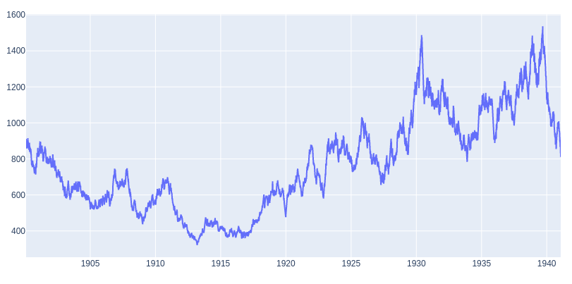
Figure 1 shows an example synthetic series with an Auto Correlation Function (ACF) realized of $0.1539$, and my model parameters were mean $\mu=0$, correlation $\rho = .15$, and 15000 samples or trading days. So there is variance around my expected parameters due to the random Gaussian distribution; however, it does come out relatively well. Although the returns do not have an underlying positive bias due to $\mu=0$, the autocorrelation alone creates ‘trends.’ This compounding effect also creates different types of ‘trends’ some fast and sharp (e.g., 1927 - 1931), some slow and steady (e.g., 1900 to 1905), and spectacular crashes (e.g., 1939-1941).
Aside: Why use synthetic data?
Synthetic data is an essential tool, especially when working with datasets that have limited historical sources. For example, emerging markets, cryptocurrencies, or exotic markets. I believe this is the most commonly thought of usage. However, one that is highly underestimated is the ability to create ‘laboratory’ like conditions, especially in financial time series. Financial time series are complex adaptive systems with various agents and are exceedingly difficult to model. This reason is why most prefer to use only actual historical data. However, this has another drawback other than historical data duration. Due to the multitude of agents' nature, actions/reactions, feedback loops, and adaptivity, it can be challenging to disentangle why a specific strategy may work. Regressions can help isolate the percentage of which factors affect your strategy or drive the time series at a specific timeframe; however, the factors will be mixing in a constantly shifting way. Although pure market replication is something that I think machine learning and generative adversarial networks may help in the future. That is not what I am trying to do here.
I am creating a purely synthetic dataset that exhibits attributes of the actual dataset. However, it is simplified as all models are. The benefit to the researcher is the control over the parameters, e.g., length, volatility, autocorrelation, as we have used here. Working as a quantitative researcher in a noisy environment makes disentangling confounding factors extremely difficult. By isolating the parts of the stochastic process, I find important and creating a clean environment tuned to create both beneficial and harsh situations for my hypothesis. I can do two things. First, remove confounding factors, so I know that I am testing against removing noise from my results. Second, able to determine boundary conditions to my thesis by expanding underlying timeseries parameters beyond normal conditions.
The Random Entry and Trailing Exit
Our “trading strategy,” if we can call it that uses a random number generator (Numpy’s implementation) to “flip a coin,” with parameters $\ge .50$ is long, and $<.50$ is short. This $\ge$ does introduce some bias, although minimal would occur when the float conversion of .50 and the randomly generated digit to 8 decimals is precisely the same. The system will take a random entry on day one. If it is closed by the trailing stop at any point on the next day, it will flip again. Someone in Jerry Parker’s clubhouse mentioned a potential bias with this method, that you would be taking a ‘pull back’ or mean reversion trade upon instant reentry. I do not have the source material. However, I disagree as, over many trials, you will end up with an equal amount of trades that go in the same direction as those in the opposite direction.
Detailing the exit is straightforward. I use a price-based standard deviation with a look back and a multiplier (e.g. 30 days look back and 3 x multiplier). If the closing price of a given day is below (above) on the next day, I exit at that day’s closing price. This does add an element of slippage, and again due to many trials should equalize. The two free parameters in this strategy is the look back for price standard deviation and its multiplier.
Below is a chart with arbitrary sample parameters for illustration.
Figure 2: Random entry and trailing exit on synthetic series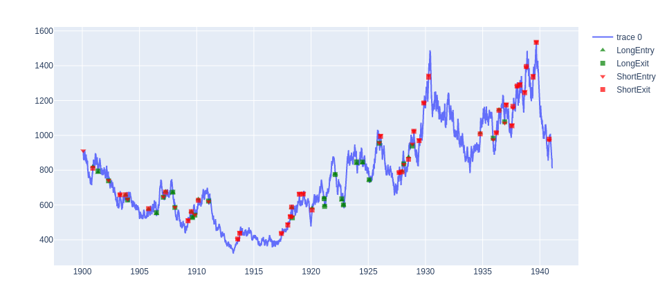
Figure 3: Zoom in on Figure 2 for detail
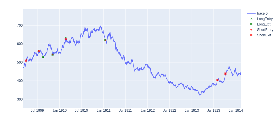
In Figure 3 we can see a better representation of both choppy markets (1909-1911) where the system is continually reversing or has a long trade that ends as a small loser in Jan 1911. As well as a long term trend trade from Jan 1911 short to the closing in Jul 1913.
What is the actual characteristics of real markets?
Let us examine some actual futures markets and see what are the real results for drift (annualized return), volatilty (annualized volatility) and Auto Correlation Function at lag 1 $ACF(1)$. For those who are familiar with these markets it may give some insight, and allow you to get a better idea of what the values in the synthetic data are similar to. It will also give us a base parameters we can use when we do our parameter sweep later on. I use all of the data listed above.
Table 2: Statistical Characteristics of the Futures Markets
| ES | C | CL | GC | EC | TY | |
|---|---|---|---|---|---|---|
| Drift (Ann. Returns) | 0.059075 | 0.031330 | 0.072193 | 0.076905 | 0.002254 | 0.007233 |
| Volatility (Ann. Volatility) | 0.196534 | 0.278543 | 0.789726 | 0.171488 | 0.092891 | 0.063090 |
| ACF(1) | -0.093291 | 0.023938 | 0.241062 | 0.002788 | 0.003363 | 0.002818 |
The S&P 500 (ES) and Crude Oil (CL) are pretty natural to create that mental link. S&P 500 has a positive drift or average annualized return of 5.9% over the period while Crude Oil was at 7.2%. ES has an annualized volatility of about 20%, while CL is much higher at 79%. The ACF is a bit harder as people do not usually think in these terms. For any next day in ES, there is a higher chance of mean reversion (i.e., a positive day is followed by a negative day, vice versa). At the same time, CL has a higher tenancy towards trending (i.e., a positive (negative) day is followed by a positive (negative) day.)
A question to the reader, does that ‘feel’ like your experience?
Random Entry / Trailing Stop on Real Markets
Here we will test the trade statistics of the trading entry and exits as done above. The parameter sets again were chosen arbitrarily as a middle of the road. Our strategy does differ from the original Van Tharpe/Tom Basso in the parameters chosen. However, we are here to prove a robust theory. So it should show similar results given any minor deviations from the original piece. My purpose here is not to prove it is profitable or not, although it would be great if it were. Nevertheless, check our original three hypotheses and see if we can verify the work already done many decades ago.
Figure 4: Random System applied to ES
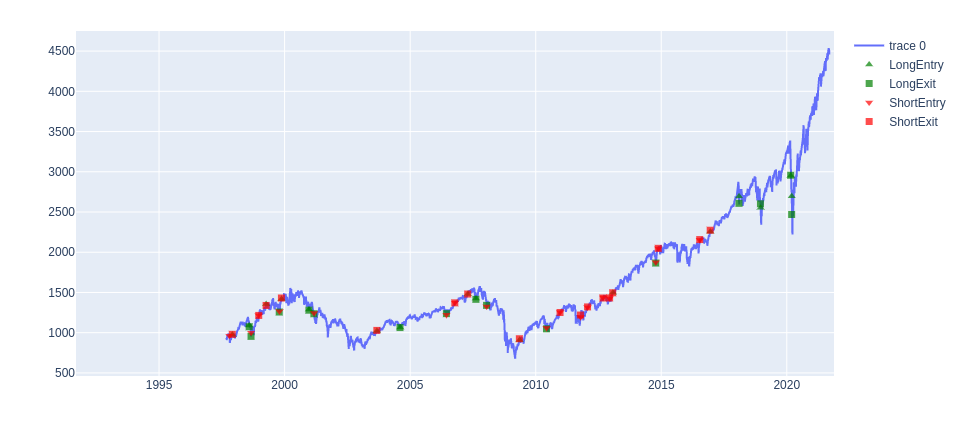
I do not give the multipliers of each future, but only the amount of spot equivalent. That is 1 dollar of profit or loss per point. I have also added the previously found ACF values for reference.
| ES | C | CL | GC | EC | TY | |
|---|---|---|---|---|---|---|
| Average Trade | -18.70 | -1.89 | 0.09 | 24.08 | 0.01 | -0.76 |
| Average Win | 203.02 | 109.49 | 14.97 | 154.51 | 0.10 | 5.14 |
| Average Loss | -134.85 | -83.07 | -12.31 | -66.22 | -0.06 | -4.13 |
| Trades Taken | 32 | 20 | 33 | 22 | 23 | 22 |
| ACF(1) | -0.093291 | 0.023938 | 0.241062 | 0.002788 | 0.003363 | 0.002818 |
The apparent issue with this test is that the sample size is too small. Each asset has a handful of trades ranging from 20 to 33. Total, we have a sample of 152 trades, which is mediocre. Let us revisit the first two of the three hypothesis statements.
-
Trailing stop losses provide an edge in autocorrelated markets.
-
- Our only example of a negatively autocorrelated market is not profitable when measured by average trade. Our most autocorrelated market is. The rest are borderline and cannot tell given sample size. I am inclined to say there is something, but more work is needed—specifically more samples.
-
Trailing stop losses alter the trade profit statistics into positive skew (bigger winners than losers).
-
- This positive skew hypothesis has been borne out of the results. All assets have a larger Average Win than Average Loss.
Hence questions remain, we must be able to expand the sample size to further answer hypothsis one. Secondly we were unable to touch hypthesis 3 because the volatilities of each asset class are drasticly different and it requires a parameter sweep.
Synthetic Data Monte Carlo
I will run 1500 runs per set, with 15000 samples or ‘days,’ which creates 22,500,000 trading days per parameter combination. With an autocorrelation value ranging from 0 to .30, stop multiplier values (i.e., how many standard deviations) from 0 to 10, and annualized volatility values from 0 to 50. As this is a multidimensional parameter sweep and it is hard to see all in a chart visually, I will go after each of our hypotheses with a set of charts and provide insight as we go along.
In regards to the number of trades per parameter combination, this is highly variable for each run given entry and exit timing as well as the set of time series parameters to the underlying we apply ranging from 0 to 1,332, with a median of 218 with a total sum of 168,436 trades recorded. This number could be improved with additional compute power and time to increase sample size infinitely. Although with median 10x improvement of sample size and confidence to real markets, I believe makes it reasonable for our uses here.
Note that we are not changing the drift parameter of the series for these tests. The autocorrelation in the market will create some natural drift component if we measure it as we did for the actual assets. However, I do not want to confound the autocorrelation effect as the drift will create a bias that will increase autocorrelation in the same direction as the drift.
Hypothesis 1: Trailing stop losses provide an edge in autocorrelated markets.
To test this, we will look at different levels of autocorrelation. First, the aggregate Average Trade value is -6.12, so we can say very definitively that a random strategy with stop loss over many trials in a pure autocorrelation environment is not the explanatory factor.
I inspect the relationship of the Average Trade (avgTrade) and the Average Winner/ Average Loser (WLRatio) in relation to the amount of autocorrelation in the series.
Figure 5: Average Trade wrt. AutoCorrelation Factor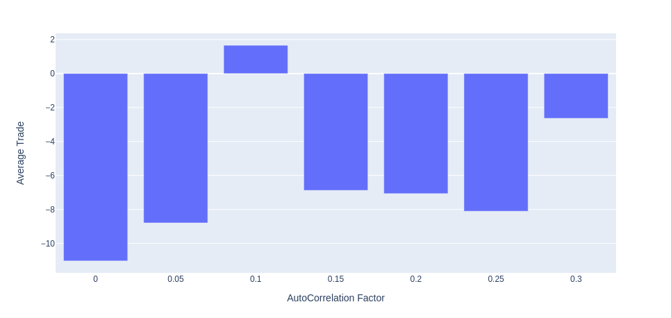
Figure 5 shows that no, autocorrelation does not provide a pure edge with a trailing stop. The outlier is the .10 positive value, but all other values are negative. With this data, I have to conclude that Hypothesis 1 is false and reject the hypothesis. That does not mean there is not anything that can be learned. Potentially there is an optimal amount of autocorrelation. The smallest autocorrelation values, 0 and 0.05, had the worst performance while adding more reduced it. Also, large amounts like 0.3 did seem to have a positive effect. Some further work could be adding the effect of an underlying drift, which all of the actual asset markets do have. This drift would amount to having a long-term memory in the underlying stochastic process.
Hypothesis 2: Trailing stop losses alter the trade profit statistics into positive skew (bigger winners than losers)
I will aggregate the win loss ratio (i.e., the average winning trade / average losing trade) from the total of all potential combinations and look at the results. For all parameter sets the mean win loss ratio was 1.73.
I have created 3d surface plots of 3 sample sets for 1, 5 and 10 precent standard deviation stop losses. For clarity the x axis autocorrelation values ranging from 0 to .30, the y axis is annualized volatility form 0 to .30. (it actually is only approaching 0 $ < 1*10^{-8}$). There is a contour line at 1 where the average winner = the average loser.
Figure 6: 1 multiplier percent Standard Deviation trailing stop loss
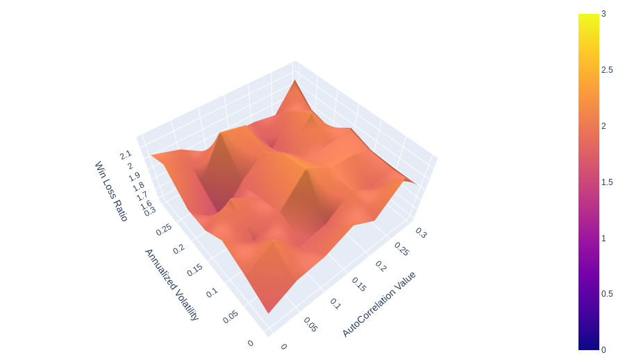
Figure 7: 5 multipler Percent Standard Deviation trailing stop loss
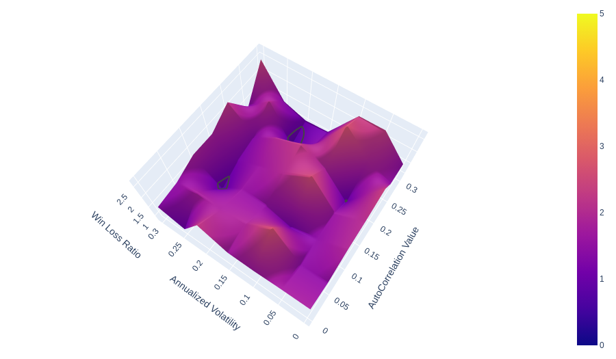
Figure 8: 10 multipler Percent Standard Deviation trailing stop loss
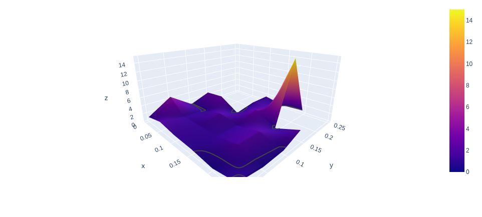
We can see that the majority of all surface areas in all three figures is above the grey contour line at 1. As we increase in multiplier we begin to see more and more surface with less than 1.
Figure 9: Trade Proft and Loss Box Plot
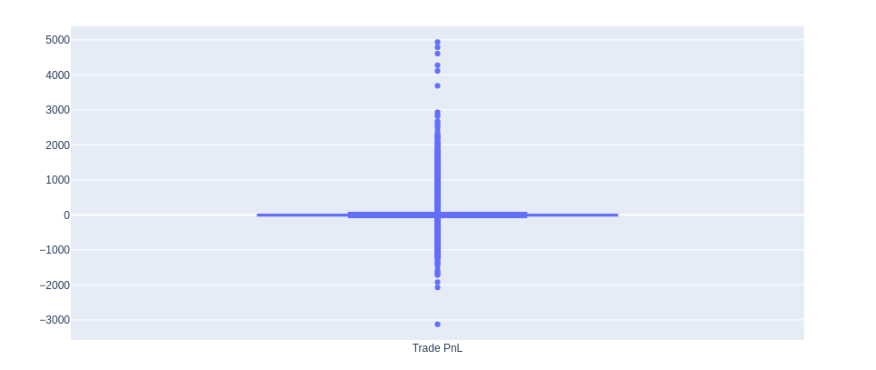
Figure 9 plots all trades taken for all simulations and parameter sets (168436 trades). This distribution was so wide due to many outliers in the distribution compared to the inner quartiles. What I can see here is that all trades have a positive skew. The skew from all trades is 6.55.
Given this information, I accept Hypothesis 2 as true. The distribution is significantly different from a normal distribution of random Trade P&Ls. Trailing stops undoubtedly alter the shape of trade results. They are cutting losers and letting winners run. Something heavily discussed is do trend following systems that use a trailing stop create an option like payoffs. From what we have here, we can only answer a partial yes. We can only address the limited downside with an upside positively skewed payoff. We cannot answer anything about convexity. We cannot measure these trade returns against something else as the trade return P&L would also be the instrument P&L less one day lag. If you look at research discussing CTA convexity, it is always in relation to the S&P 500 or other benchmarks. For the simulated data, we have no such benchmark.
Hypothesis 3: Trailing stops distance from entry become negative expected value if it is “too close.”
Here I take the average of all Average Trade values with respect to annualized volatility and the stop multiplier value. This means we are aggregating all of the auto correlation values together.
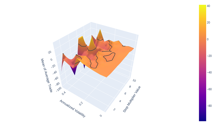
!Looking across the 2 stop multiplier level vs. the 10 levels, the decay into the trough as designated by the contour line at 0 does show a faster decay of positive average trade for smaller stop multiplier values. I cannot say that anything going towards the left cannot be profitable. It only looks to become much more unstable. At the same time, larger stop values are more stable for more values of levels of annualized volatility. I have to reject Hypothesis 3 due to the lack of conclusive results. There is some instability, but it may be possible to find small stop multiplier values profitable in some situations. There is also the confounding factor of Auto Correlation which we check below.
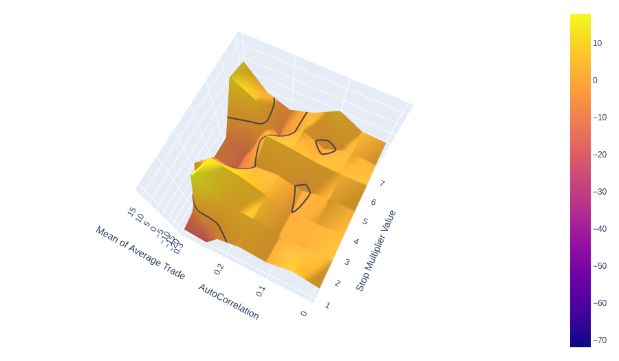
We see something interesting here, which I did not expect but intuitively makes sense. Smaller stop values work well with high amounts of autocorrelation. They can outperform the larger stop values. This effect is because, in higher autocorrelated markets, you can take less risk and loss less at the top of a trend than with a larger stop, thus catching more of the move for less risk. This only occurs because the signal-to-noise ratio is higher. This effect could be pumping up the low stop multiplier values in our other mean of average trade metrics.
Conclusion
I examined the effect of autocorrelation and volatility on random entries and trailing stop losses. I recreated a similar system to the Tom Basso/Van Tharpe method to proxy what I was doing with the synthetic data. By using synthetic data with controllable parameters, I could disentangle autocorrelation from drift and other factors present in actual market data.
On the proxy Tom Basso system, I found that random entries with a trailing stop can be profitable on highly autocorrelated assets like CL and slightly autocorrelated assets like GC. However, on negatively autocorrelated asset ES, it was negative. In the end, we ended up 50% profitable and 50% unprofitable.
I tested Hypothesis 1: Trailing stop losses provide an edge in autocorrelated markets. After many Monte Carlo simulations using the AR(1) process, we found that trailing stops are not a definitive way to increase your Average Trade. There is some evidence that more autocorrelation can lift values but not definitively make them positive. Thus I rejected the hypothesis.
For Hypothesis 2: Trailing stop losses alter the trade profit statistics into positive skew (bigger winners than losers). I definitively showed that all trades, on average, had larger winners than losers for a 1.73 Win-Loss Ratio. This is the most apparent evidence of trailing stops being the bedrock of any trend following strategy. It also clearly shows how it can alter your trade profits by skewing them positively. Hence, I accepted the hypothesis.
Finally, Hypothesis 3: Trailing stops distance from entry become negative expected value if it is “too close.” Again I did not have a definitive answer, also rejecting the hypothesis. Nevertheless, all was not lost. I learned something that should have been intuitive and may have been a confounding factor in the results. When assets are highly autocorrelated, smaller stop values are better due to their ability to take and hold positions with less risk and lose fewer profits at the top. This is because, in essence, a higher autocorrelation value is a higher signal-to-noise ratio.